
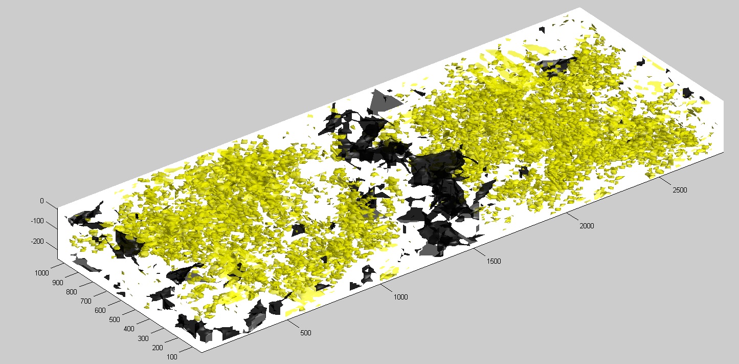
Kras mutation in 3D, mouse 176_14_2.
Mutant fraction of Kras exon 1 otained from 458 laser capture micro dissected samples used to construct a distribution of mutated alleles in 3D. The tissue is from a chemical induced mouse (FVB_NJ) mammary tumor.
Spreading 21cells based on the mutant fraction of the sampled area. Mutated cells (Yellow) or wildtype (Black).
Volume analysed 3000mm x 1200mm x 250mm
Matlab Script
tx=0:18:3000;
ty=0:18:1200
tz=-250:6:12
[xg,yg,zg] = meshgrid(tx,ty,tz);
% Interpolation method.;
F.Method = 'natural';
% The scatteredInterpolant class supports scattered data interpolation in 2-D and 3-D space.;
% Use of this class is encouraged as it is more efficient and readily adapts to a wider range of interpolation problems.;
% Create the interpolating object
F = TriScatteredInterp(x, y, z, e);
% Do the interpolation
eg = F(xg,yg,zg);
% Now you can use isosurface with the gridded data
f1=isosurface(xg,yg,zg,eg,0);
f2=isosurface(xg,yg,zg,eg,1);
%Plotting the mesh in matlab
p = patch(f1);
set(p,'FaceColor',[0 0 0],'EdgeColor','none', 'facealpha',0.4);
p = patch(f2);
set(p,'FaceColor',[1 1 0],'EdgeColor','none', 'facealpha',0.4);
daspect([1 1 1]); view(3); axis tight; camlight; lighting gouraud;
% The script figure2xhtml generates the 3D interactive rendering.
figurexhtml
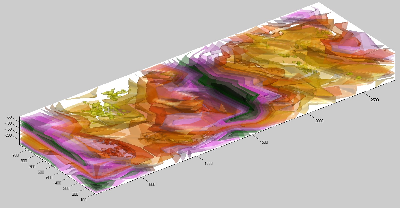
Alternative way of displaying the data: Scale x, y, z in micro meter, colors of mutant fraction from 0 to 100%.
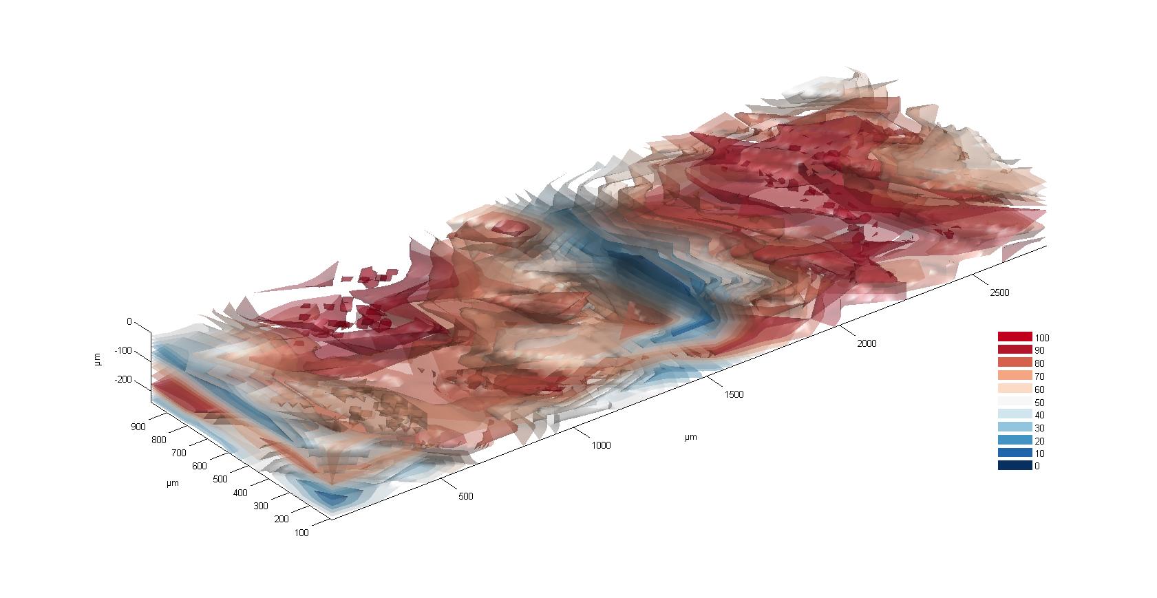
Distribution of mutant fractions from 0% (Black) up to 100% (Yellow).
Matlab script used to genered the Html file.
tx=0:18:3000;
ty=0:18:1200
tz=-250:6:12
[xg,yg,zg] = meshgrid(tx,ty,tz);
% Interpolation method.;
F.Method = 'natural';
% The scatteredInterpolant class supports scattered data interpolation in 2-D and 3-D space.;
% Use of this class is encouraged as it is more efficient and readily adapts to a wider range of interpolation problems.;
% Create the interpolating object
F = TriScatteredInterp(x, y, z, e);
% Do the interpolation
eg = F(xg,yg,zg);
% Now you can use isosurface with the gridded data
f1=isosurface(xg,yg,zg,eg,0.1);
f2=isosurface(xg,yg,zg,eg,0.2);
f3=isosurface(xg,yg,zg,eg,0.3);
f4=isosurface(xg,yg,zg,eg,0.4);
f5=isosurface(xg,yg,zg,eg,0.5);
f6=isosurface(xg,yg,zg,eg,0.6);
f7=isosurface(xg,yg,zg,eg,0.7);
f8=isosurface(xg,yg,zg,eg,0.8);
f9=isosurface(xg,yg,zg,eg,0.9);
f10=isosurface(xg,yg,zg,eg,1);
%Plotting the mesh in matlab
p = patch(f1);
set(p,'FaceColor',[0 0 0],'EdgeColor','none', 'facealpha',0.4);
p = patch(f2);
set(p,'FaceColor',[0 0.25 0],'EdgeColor','none', 'facealpha',0.4);
p = patch(f3);
set(p,'FaceColor',[0 0.5 0],'EdgeColor','none', 'facealpha',0.4);
p = patch(f4);
set(p,'FaceColor',[1 0.25 1],'EdgeColor','none', 'facealpha',0.4);
p = patch(f5);
set(p,'FaceColor',[1 0.5 1],'EdgeColor','none', 'facealpha',0.4);
p = patch(f6);
set(p,'FaceColor',[1 0.75 1],'EdgeColor','none', 'facealpha',0.4);
p = patch(f7);
set(p,'FaceColor',[1 0.25 0],'EdgeColor','none', 'facealpha',0.4);
p = patch(f8);
set(p,'FaceColor',[1 0.5 0],'EdgeColor','none', 'facealpha',0.4);
p = patch(f9);
set(p,'FaceColor',[1 0.75 0],'EdgeColor','none', 'facealpha',0.4);
p = patch(f10);
set(p,'FaceColor',[1 1 0],'EdgeColor','none', 'facealpha',0.4);
daspect([1 1 1]); view(3); axis tight; camlight; lighting gouraud;
%generate html file
figure2xhtml